Need help? Have a feature request? Please check out the tethne-users group .

Generating and Visualizing Topic Models with Tethne and MALLET¶

Before You Start
Loading JSTOR DfR
- Using a Stoplist
- Checking your Data
Filtering words
Topic Modeling in MALLET
Inspecting the Model
- Topics over Time
Semantic Graph
- Build the Network
- Visualization
Wrapping up, Looking forward

Note

This tutorial was developed for the course Introduction to Digital & Computational Methods in the Humanities (HPS), created and taught by Julia Damerow and Erick Peirson.

Tethne provides a variety of methods for working with text corpora and the output of modeling tools like MALLET. This tutorial focuses on parsing, modeling, and visualizing a Latent Dirichlet Allocation topic model, using data from the JSTOR Data-for-Research portal.

In this tutorial, we will use Tethne to prepare a JSTOR DfR corpus for topic modeling in MALLET, and then use the results to generate a semantic network like the one shown below.

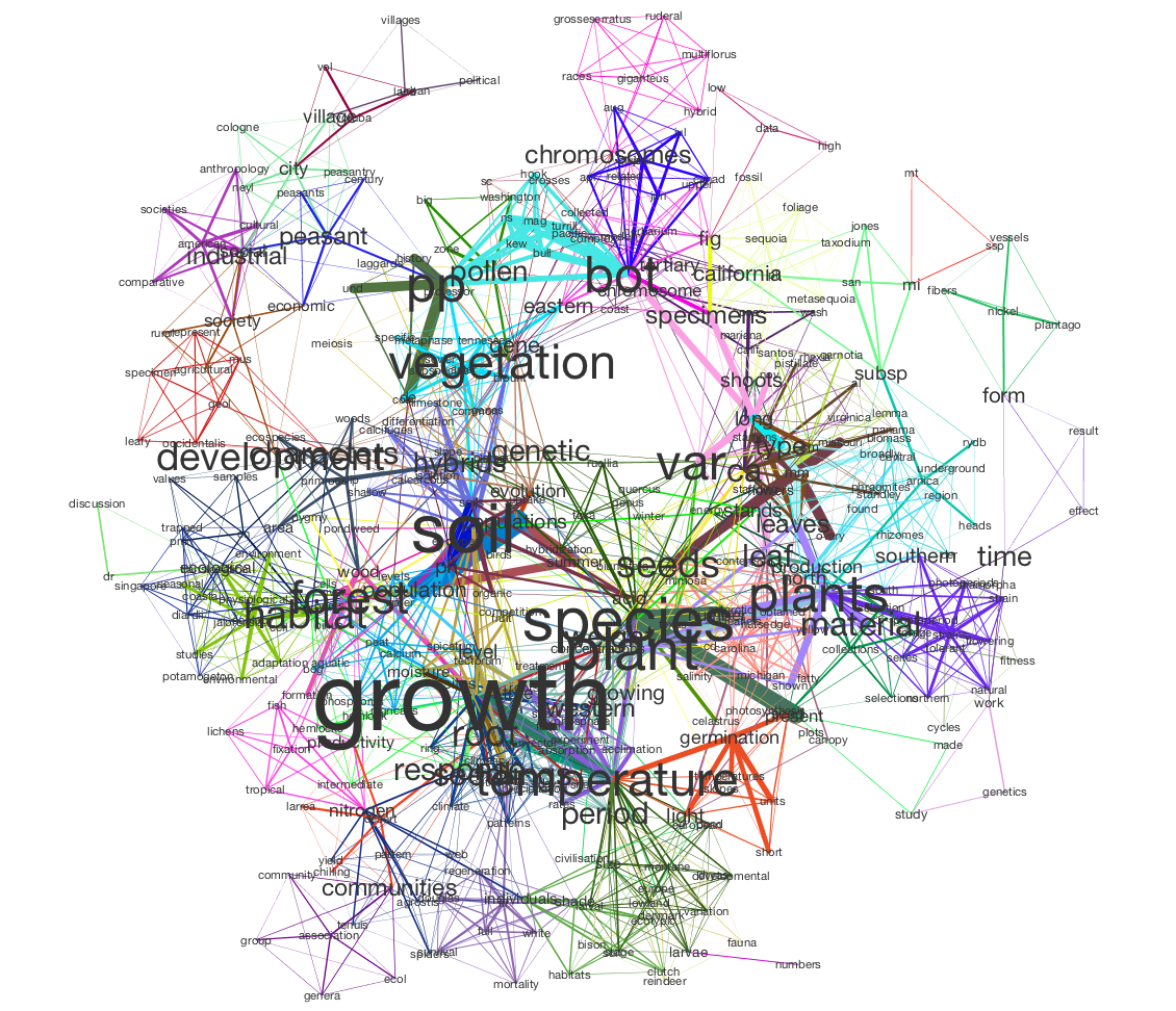
In this visualization, words are connected if they are associated with the same topic; the heavier the edge, the more strongly those words are associated with that topic. Each topic is represented by a different color. The size of each word indicates the structural importance (betweenness centrality) of that word in the semantic network.

This tutorial assumes that you already have a basic familiarity with Cytoscape.

Before You Start ¶

You’ll need some data. See JSTOR Data-for-Research for instructions on retrieving data. Note that Tethne currently only supports XML output from JSTOR. Be sure to get some wordcounts so that you’ll have some data for modeling.

Be sure that you have the latest release of Tethne. See installation.

You should also download and install MALLET.

Loading JSTOR DfR ¶

Use the readers.dfr module to load data from JSTOR DfR. Since we’re working with a single DfR dataset that contains wordcounts, we’ll use the dfr.read() method.

Assuming that you unzipped your JSTOR DfR dataset to /Users/me/JStor DfR Datasets/2013.5.3.cHrmED8A, you can use something like the following to generate a Corpus from your dataset:

>>> from tethne.readers import dfr
>>> datapath = '/Users/me/JStor DfR Datasets/2013.5.3.cHrmED8A'
>>> corpus = dfr.read(datapath, streaming=True, index_fields=['date', 'abstract'], index_features=['authors'])

By default, the DfR reader will look for unigrams in your dataset, and load them up as a featureset. Depending on the size of your dataset, this might take a few moments. The reader will attempt to discard junk data (e.g. unigrams with hashes ### in them), and index all of the Papers and features in the dataset.

Using a Stoplist ¶

You may want to pare down our dataset further still, by applying a list of stop words. We can achieve this using a “transformation” of the original wordcounts.

First, load the NLTK stoplist:

>>> from nltk.corpus import stopwords
>>> stoplist = stopwords.words()

stoplist is just a list of words. You can add words by ``append()``ing them, remove words, or create your own list from scratch.

>>> mystoplist = ['words', 'that', 'bother', 'me']

We’ll apply the stoplist by defining a transformation. A transformation is just a function that accepts some feature (word)-specific parameters, and returns a value for that feature. This will be applied to every word in every document. In particular, the transformation will receive four pieces of information:

A token of the feature (usually a str or unicode),
The document-specific value (e.g. word count),
The corpus-wide value (e.g. word counts for the corpus),
The number of documents in which the feature occurs.

In this case, we want to evaluate whether or not the token comes from our stop list and, if it does, return None so that the word is removed.

>>> def apply_stoplist(token, count, global_count, document_document):
...     if token in stoplist:
...         return None    # Tells Tethne to remove the word.
...     return count    # If we get to here, the word wasn't in the list.

Then we’ll create a new FeatureSet using that transformation. The actual .transform() step may take a minute or two, depending on the size of your collection.

>>> wordcounts = corpus.features['wordcounts']
>>> wordcounts.top(5)    # Before the transformation.
[('the', 171147.0), ('of', 147276.0), ('and', 86814.0), ('in', 79627.0), ('a', 50211.0)]

>>> wordcounts_filtered = wordcounts.transform(apply_stoplist)
>>> wordcounts_filtered.top(5)    # After the transformation.
[('species', 13417.0), ('p', 7037.0), ('plants', 6901.0), ('x', 6559.0), ('may', 6315.0)]

>>> corpus.features['wordcounts_filtered'] = wordcounts_filtered

That last step is important, as it keeps all of our feature data organized in our Corpus.

Checking your Data ¶

If everything goes well, you should have a Corpus with some Papers in it...

>>> corpus
<tethne.classes.corpus.Corpus object at 0x108403310>

>>> len(corpus)
241

...as well as a FeatureSet called wordcounts_filtered:

>>> corpus.features.keys()
['wordcounts', 'wordcounts_filtered']

>>> len(corpus.features['wordcounts_filtered'].index')       # Unique features (words).
51693

Some of your papers may not have wordcounts associated with them. You can check how many papers have wordcount data:

>>> len(corpus.features['wordcounts_filtered'].features)
193

Filtering words ¶

In the previous section, you loaded some DfR data with wordcounts (unigrams). That resulted in a Corpus with a featureset called wordcounts_filtered, containing 51,639 unique words. That’s a lot of words. Using a large vocabulary increases the computational cost of building and visualizing your model. There may also be quite a few “junk” words left in your vocabulary. We can use the same procedure that we used above – applying a transformation – to further refine our data.

The transformation below will remove any words that are shorter than four characters in length, occur less than four times overall, and are found in less than two documents.

>>> def filter(f, c, C, DC):
...     if C < 4 or DC < 2 or len(f) < 4:
...         return None
...     return c

Once your transformation is defined, call FeatureSet.transform(), just like last time:

>>> wordcounts_filtered = corpus.features['wordcounts_filtered']
>>> wordcounts_filtered.top(5)    # Before the transformation.
[('species', 13417.0), ('p', 7037.0), ('plants', 6901.0), ('x', 6559.0), ('may', 6315.0)]

>>> wordcounts_uberfiltered = wordcounts_filtered.transform(filter)
>>> wordcounts_uberfiltered.top(5)    # After the transformation.
[(('experimental', True), 396.0), (('taxonomy', True), 363.0), (('plant', True), 352.0), (('species', True), 347.0), (('plants', True), 330.0)]

>>> corpus.features['wordcounts_uberfiltered'] = wordcounts_uberfiltered

Your new featureset, wordcounts_uberfiltered, should be much smaller than the old featureset.

>>> len(corpus.features['wordcounts_uberfiltered'].index)
12675

In this example, only 12,675 unique words were retained. This is far more computationally tractable.

Topic Modeling in MALLET ¶

Tethne provides an interface to MALLET, so that you can fit an LDA topic model without leaving the Python environment. In the background, Tethne builds a plain-text corpus that MALLET can take as input, fits the model, and parses the results.

For details about LDA modeling in MALLET, consult the MALLET website as well as this tutorial.

Tethne ships with MALLET, so you don’t need to install anything extra.

The MALLET interface can be found in tethne.model.corpus:

>>> from tethne.model.corpus import mallet

We first need to instantiate a mallet.LDAModel with our Corpus and preferred FeatureSet.

>>> model = mallet.LDAModel(corpus, featureset_name='wordcounts_uberfiltered')

We can set the number of topics (Z, in Tethne) and the maximum number of iterations like this:

>>> model.Z = 20
>>> model.max_iter = 500    # Try starting with a low number, then go higher.

When you’re ready to fit the model, call mallet.LDAModel.fit().

>>> model.fit()
Modeling progress: 18%.

Depending on the size of the corpus, number of topics, and maximum number of iterations, this may take anywhere from a minute to an hour. Luckily there is a progress indicator to keep you entertained.

Inspecting the Model ¶

You can inspect the model using the LDAModel.print_topics() method, which prints the most likely words from each topic. You can control the number of words returned for each topic by passing the Nwords parameter.

>>> print model.print_topics(Nwords=5)
Topic        Top 5 words
  populations length characters population analysis
  airy shaw subsp hook verdc
  species vegetation forest ecological forests
  plants populations growth conditions plant
  salt leaves spray water species
  growth activity behavior animals activities
  jour studies growth plant development
  species taxonomic groups taxonomy evolution
  leaves leaf cells species upper
  work botanical names plant time
 species north subsp california lewis
 host parasites infection parasite cells
 hybrids species chromosome chromosomes hybrid
 university society state august american
 seed varieties color resistance bean
 research university department position experience
 plants plant large found number
 species utricularia long corolla upper
 species pollen british flora group
 research department university number international

To see posterior probabilities for words in a specific topic, use LDAModel.list_topic():

>>> model.list_topic(5, Nwords=20)
[(u'growth', 0.011455776240422525), (u'activity', 0.01009819236777505),
 (u'behavior', 0.009205534478910957), (u'animals', 0.00900096704604627),
 (u'activities', 0.0073644275831287655), (u'environment', 0.007271442386372089),
 (u'time', 0.006657740087778026), (u'organisms', 0.006415978576210667),
 (u'control', 0.006192814103994644), (u'occurs', 0.006137022985940638),
 (u'environmental', 0.005820873316967939), (u'water', 0.00557911180540058),
 (u'rainfall', 0.005337350293833222), (u'factors', 0.005262962136427881),
 (u'food', 0.005058394703563193), (u'tree', 0.004816633191995834),
 (u'influence', 0.004723647995239158), (u'life', 0.004463289444320465),
 (u'modification', 0.003998363460537083), (u'direct', 0.003775198988321059)]

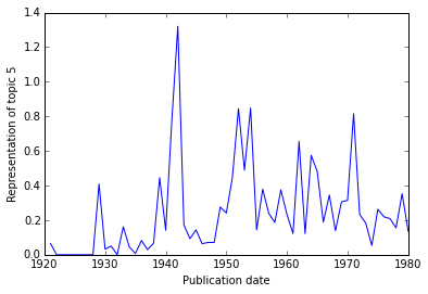
Topics over Time ¶

If your dataset contains data from a broad range of time, you may wish to visualize the representation of particular topics over time.

To obtain the representation of a topic over time, use LDAModel.topic_over_time().

>>> years, representation = model.topic_over_time(5)
>>> years    # The publication years in the corpus.
[1921, 1922, 1923, 1924, 1925, 1926, 1927, 1928, 1929, 1930, 1931, 1932,
 1933, 1934, 1935, 1936, 1937, 1938, 1939, 1940, 1941, 1942, 1943, 1944,
 1945, 1946, 1947, 1948, 1949, 1950, 1951, 1952, 1953, 1954, 1955, 1956,
 1957, 1958, 1959, 1960, 1961, 1962, 1963, 1964, 1965, 1966, 1967, 1968,
 1969, 1970, 1971, 1972, 1973, 1974, 1975, 1976, 1977, 1978, 1979, 1980]
 >>> representation   # The corresponding representation of topic 5.
 [0.06435643564356436, 0.0, 0.0, 0.0, 0.0, 0.0, 0.0, 0.0, 0.4087281927881383,
  0.0325, 0.04976303317535545, 0.0, 0.16161454631603886, 0.04484382804857306,
  0.006614360003649302, 0.08236126314837293, 0.029438839430272666,
  0.0657948892738444, 0.44573451608857595, 0.14148988107236954,
  0.7704054711026587, 1.3210010767530431, 0.17188550885325318,
  0.093189448441247, 0.14402439613999296, 0.06395882153971835,
  0.07077772475410271, 0.07098077700383691, 0.2757824307011957,
  0.24073191125669346, 0.4462418858215179, 0.8448802795214342,
  0.4889481845849125, 0.8479697688991538, 0.14351703956816014,
  0.3791279329284834, 0.23920240501357345, 0.1868955193635965,
  0.37539119354048034, 0.23301379444472836, 0.12294899401514778,
  0.6555419699902894, 0.1221671346807374, 0.5747231715488136,
  0.48069209562159615, 0.1882118294403064, 0.3451598212675003,
  0.1386416394307499, 0.3054123456539457, 0.3146222720563767,
  0.8150255574909027, 0.23251257653445442, 0.18303059584803458,
  0.05314921621305513, 0.2628134619537122, 0.21919993327260742,
  0.2088760199747929, 0.15513474090076687, 0.35286000356433866,
  0.13642535834857786]

We can easily visualize this using MatPlotLib (assuming that you’re working in IPython):

>>> import matplotlib.pyplot as plt
>>> plt.plot(years, representation)
>>> plt.xlabel('Publication date')
>>> plt.ylabel('Representation of topic 5')
>>> plt.show()   # Use .save() if you're not in IPython.

Semantic Graph ¶

In LDA, topics are clusters of terms that co-occur in documents. We can interpret an LDA topic model as a graph of terms linked by their participation in particular topics.

Build the Network ¶

We can generate the term graph using the terms() method from the networks.topics module. There are other kinds of graph-building methods in there; go check them out!

>>> from tethne.networks import topics
>>> graph = topics.terms(model, threshold=0.015)

The threshold argument tells Tethne the minimum P(W|T) to consider a topic (T) to contain a given word (W). In this example, the threshold was chosen post-hoc by adjusting its value and eye-balling the resultant network for coherence.

We can then write this graph to a GraphML file for visualization:

>>> import tethne.writers as wr
>>> wr.graph.to_graphml(graph, './mymodel_tc.graphml')

Visualization ¶

In Cytoscape, import your GraphML network by selecting File > Import > Network > From file... and choosing the file mymodel_tc.graphml from the previous step.

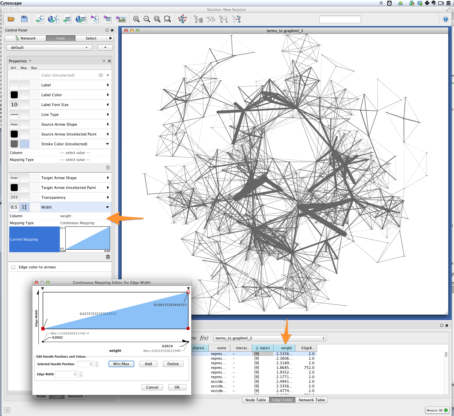
Edge weight¶

Tethne included joint average P(W|T) for each pair of terms in the graph as the edge attribute weight. You can use this value to improve the layout of your network. Try selecting Layout > Edge-weighted Spring Embedded > weight.

You can also use a continuous mapper to represent edge weights visually. Create a new visual mapping (in the VizMapper tab in Cytoscape < 3.1, Style in >= 3.1) for edge width.

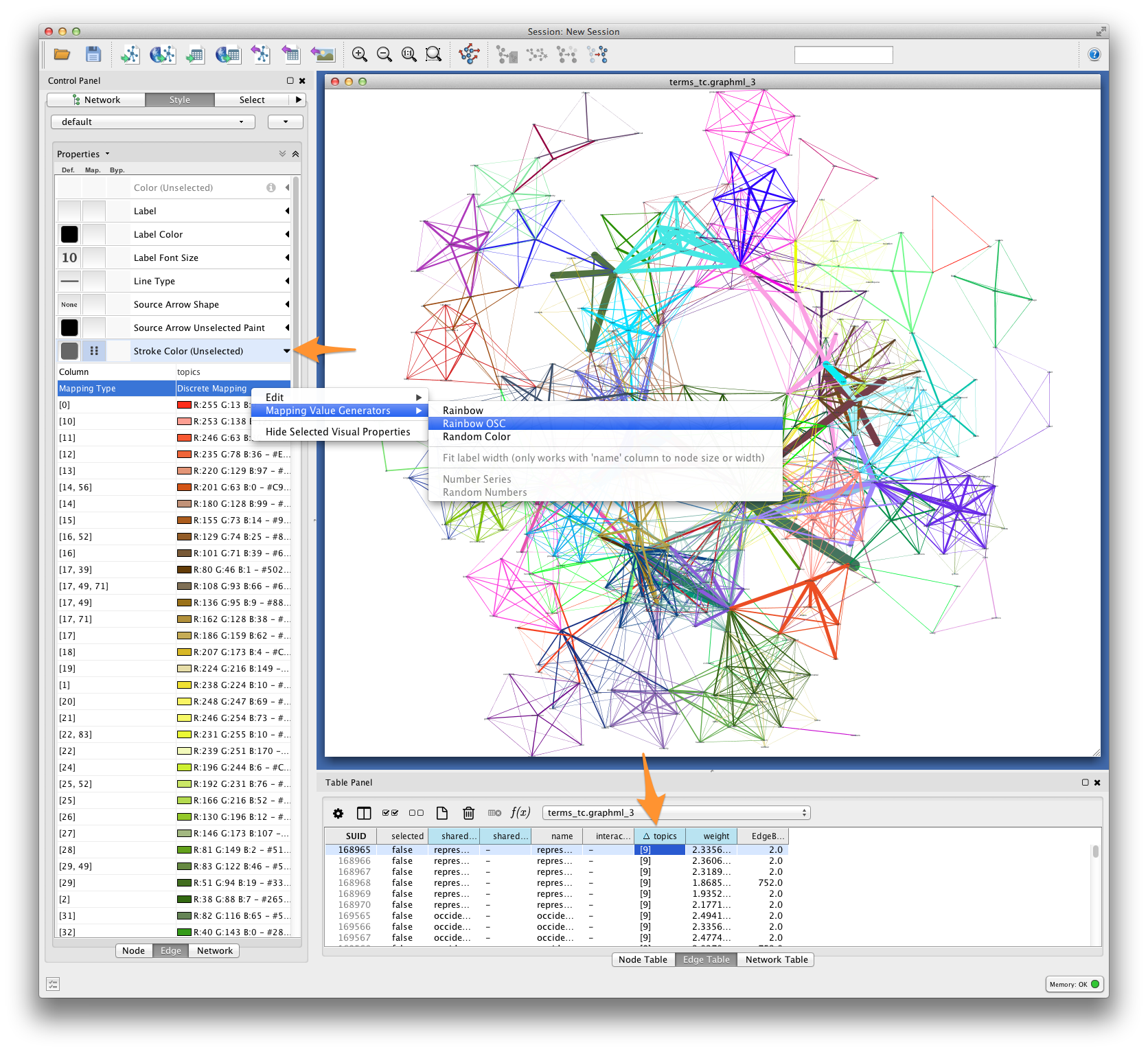
Edge color¶

For each pair of terms, Tethne records shared topics in the edge attribute topics. Coloring edges by shared topic will give a visual impression of the “parts” of your semantic network. Create a discrete mapping for edge stroke color, and then right-click on the mapping to choose a color palette from the Mapping Value Generators.

Font-size¶

Finally, you’ll want to see the words represented by each of the nodes in your network. You might be interested in which terms are most responsible for bridging the various topics in your model. This “bridging” role is best captured using betweenness centrality, which is a measure of the structural importance of a given node. Nodes that connect otherwise poorly-connected regions of the network (e.g. clusters of words in a semantic network) have high betweenness-centrality.

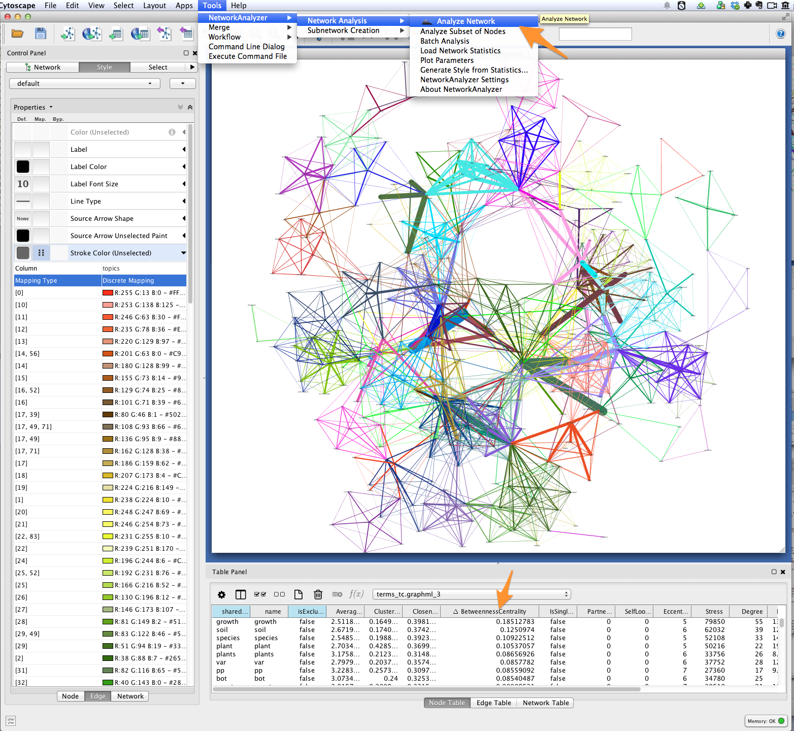
Use Cytoscape’s NetworkAnalyzer to generate centrality values for each node: select Tools > NetworkAnalyzer > Network Analysis > Analyze Network. Once analysis is complete, Cytoscape should automatically add a BetweennessCentrality node attribute to the graph.

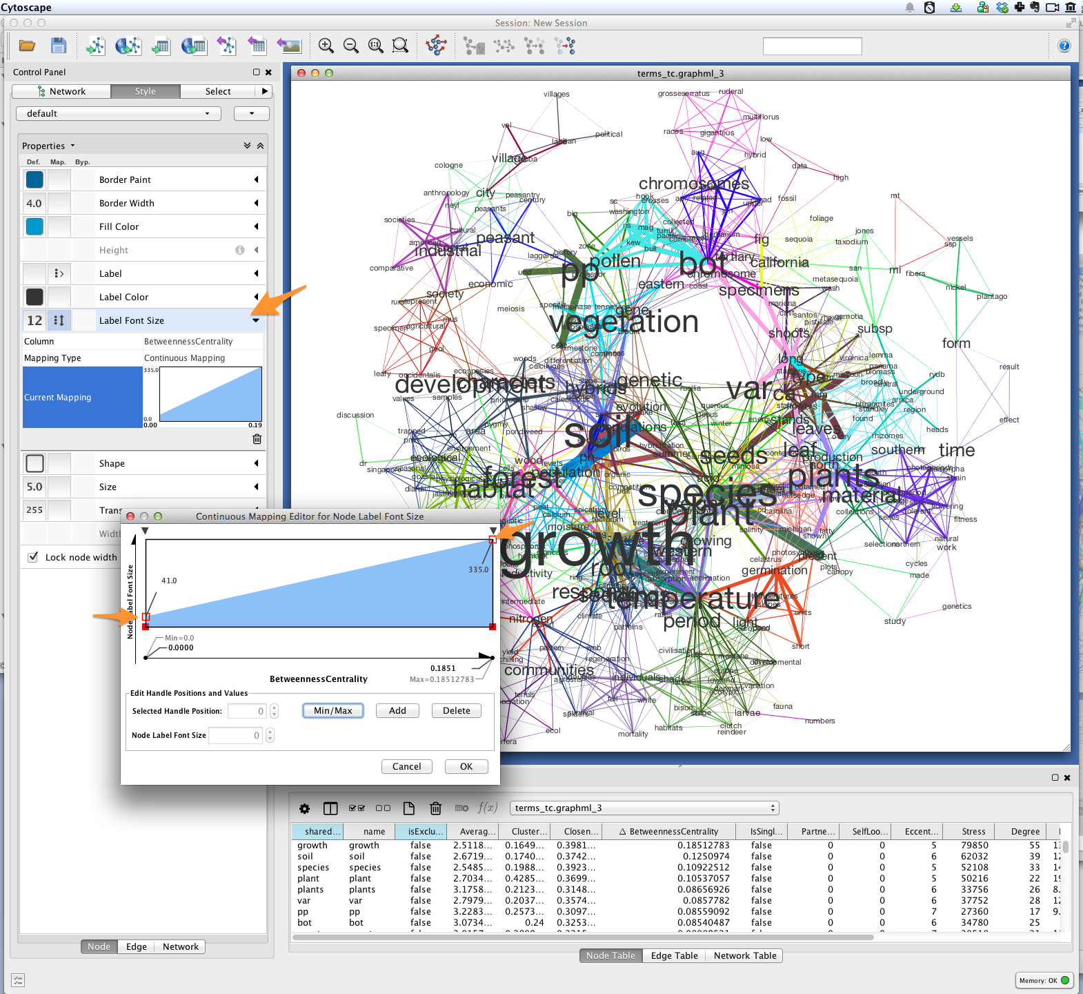
Next, create a continuous mapping for Label Font Size based on BetweennessCentrality. More central words should appear larger. In the figure below, label font size ranges from around 40 to just over 300 pt.

Export¶

Export the finished visualization by selecting File > Export > Network View as Graphics....

Wrapping up, Looking forward ¶

To generate a network of papers connected by topics-in-common, try the topic_coupling() function.

Since Tethne is still under active development, function for working with topic modeling and other corpus-analysis techniques are being added all the time, and existing functions will likely change as we find ways to streamline workflows. This tutorial will be updated and extended as development proceeds.